Analysis of categorical data generally involves the use of data tables. A two-way table presents categorical data by counting the number of observations that fall into each group for two variables, one divided into rows and the other divided into columns. For example, suppose a survey was conducted of a group of 20 individuals, who were asked to identify their hair and eye color. A two-way table presenting the results might appear as follows:
			Eye Color
Hair Color	Blue	Green	Brown	Black	Total
-----------------------------------------------------
Blonde		2	1	2	1	6
Red		1	1	2	0	4
Brown		1	0	4	2    	7
Black		1	0	2	0	3
-----------------------------------------------------
Total		5	2	10	3   	20
The totals for each category, also known as marginal distributions, provide the number of individuals in each row or column without accounting for the effect of the other variable (in the example above, the total number of individuals with blue eyes, regardless of hair color, is 5).
Since simple counts are often difficult to analyze, two-way tables are often converted into percentages. In the above example, there are 4 individuals with red hair. Since there were a total of 20 observations, this means that 20% of the individuals survered are redheads. One also might want to investigate the percentages within a given category -- of the 4 redheads, 2 (50%) have brown eyes, 1 (25%) has blue eyes, and 1 (25%) has green eyes.
For a more detailed example, consider the following dataset, "Weights of 1996 US Olympic Rowing Team." The first column gives the name of the rower, the second gives his event, and the third gives his weight. There are 8 different event categories, with weight given as numeric data.
Auth        LW_double_sculls     154	Klepacki    four                 205
Beasley     single_sculls        224	Koven       eight                200
Brown       eight                214	Mueller     quad                 215
Burden      eight                195	Murphy      eight                220
Carlucci    LW_four              160	Murray      four                 205
Collins,D   LW_four              155	Peterson,M  pair                 210
Collins,P   eight                195	Peterson,S  LW_double_sculls     160
Gailes      quad                 205	Pfaendtner  LW_four              160
Hall        four                 195	Schnieder   LW_four              158
Holland     pair                 195	Scott       four                 208
Honebein    eight                200	Segaloff    coxswain             121
Jamieson    quad                 210	Smith       eight                207
Kaehler     eight                210	Young       quad                 207
Data source: Team member biographies given on the NBC Olympic Web Site. Dataset available through the JSE Dataset Archive.
Descriptive Statistics

Variable        N     Mean   Median  Tr Mean    StDev  SE Mean
Weight         26   191.85   202.50   193.46    26.27     5.15

Variable      Min      Max       Q1       Q3
Weight       121.00   224.00   160.00   210.00
One might choose, based on this information, to divide the weight values into 4 groups, such as under 150 lbs, 150-175 lbs, 175-200 lbs, and over 200 lbs. Once the data has been categorized (the MINITAB "CODE" command may be used to perform this function), the MINITAB "TABLE" command will create two-way tables, as follows:
 Rows: Event     Columns: Weight_Class

              <150    150-175   175-200  >200      All

 LW_doubl       0        2        0        0        2
 single_s       0        0        0        1        1
 eight          0        0        4        4        8
 LW_four        0        4        0        0        4
 quad           0        0        0        4        4
 four           0        0        1        3        4
 pair           0        0        1        1        2
 coxswain       1        0        0        0        1
 All            1        6        6       13       26
Using the "ROWPERCENT" subcommand reproduces this table with the percentages of rowers in each
weight category by event:
 Rows: Event     Columns: Weight_Class

                0        1        2        3      All

 LW_doubl     --    100.00      --       --    100.00
 single_s     --       --       --    100.00   100.00
 eight        --       --     50.00    50.00   100.00
 LW_four      --    100.00      --       --    100.00
 quad         --       --       --    100.00   100.00
 four         --       --     25.00    75.00   100.00
 pair         --       --     50.00    50.00   100.00
 coxswain  100.00      --       --       --    100.00
 All         3.85    23.08    23.08    50.00   100.00
These results indicate that half of all rowers are in the upper weight class, with the remainder
evenly divided between the two middle classes (with the exception of the coxswain, who is the only
team member in the lightest weight group). Similarly, the "COLPERCENT" subcommand provides the
percentage of rowers in each event category by weight.

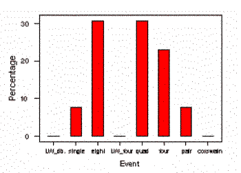
In addition to creating data tables, an analyst might want to create a graphical representation of categorical data using a bar graph. A bar graph representing the percentage of rowers in the heaviest weight category in each event is shown to the left.

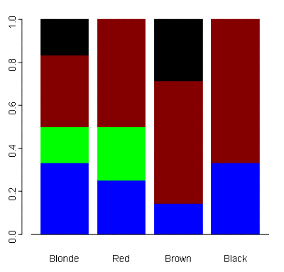
Another useful graphical tool for analyzing categorical data is a segmented bar graph. For the simple hair color/eye color example above, a segmented bar graph depicting the breakdown of eye color for each hair color appears to the right. The segments of each bar are color-coded to correspond to the appropriate eye color.