The Normal Distribution

A normal distribution has a bell-shaped density curve described by its mean

and standard deviation

. The density curve is symmetrical, centered about its mean, with its spread determined by its standard deviation. The height of a normal density curve at a given point x is given by

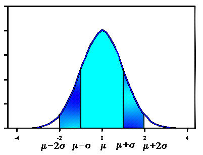
The Standard Normal curve, shown here, has mean 0 and standard deviation 1. If a dataset follows a normal distribution, then about 68% of the observations will fall within of the mean , which in this case is with the interval (-1,1). About 95% of the observations will fall within 2 standard deviations of the mean, which is the interval (-2,2) for the standard normal, and about 99.7% of the observations will fall within 3 standard deviations of the mean, which corresponds to the interval (-3,3) in this case. Although it may appear as if a normal distribution does not include any values beyond a certain interval, the density is actually positive for all values, . 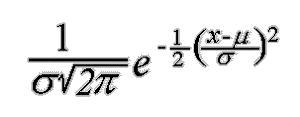Data from any normal distribution may be transformed into data following the standard normal distribution by subtracting the mean and dividing by the standard deviation .

Example

The dataset used in this example includes 130 observations of body temperature. The MINITAB "DESCRIBE" command produced the following numerical summary of the data:

Variable        N     Mean   Median  Tr Mean    StDev  SE Mean
BODY TEMP      130   98.249   98.300   98.253    0.733    0.064

Variable      Min      Max       Q1       Q3
BODY TEMP    96.300  100.800   97.800   98.700

The spread of the data is very small, as might be expected.

The normality of the data may be evaluated by using the MINITAB "NSCORES" command to calculate the normal scores for the data, then plotting the observed data against the normal quantile values. For the first 10 sorted observations, the table below displays the original temperature values in the first column, standardized values in the second column (calculated by subtracting the mean 98.249 and dividing by the standard deviation 0.733), and corresponding normal scores in the third column.

96.3	-2.65894	-2.58163
96.4	-2.52251	-2.24352
96.7	-2.11323	-1.98066
96.7	-2.11323	-1.98066
96.8	-1.97681	-1.80820
96.9	-1.84038	-1.71725
97.0	-1.70396	-1.63847
97.1	-1.56753	-1.50561
97.1	-1.56753	-1.50561
97.1	-1.56753	-1.50561

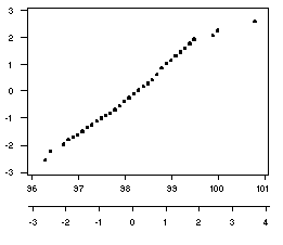The standardized values in the second column and the corresponding normal quantile scores are very similar, indicating that the temperature data seem to fit a normal distribution. The plot of these columns, with the temperature values on the horizontal axis and the normal quantile scores on the vertical axis, is shown to the right (the two scales in the horizontal axis provide original and standardized values). This plot indicates that the data appear to follow a normal distribution, with only the three largest values deviating from a straight diagonal line.

Data source: Derived from Mackowiak, P.A., Wasserman, S.S., and Levine, M.M. (1992), "A Critical Appraisal of 98.6 Degrees F, the Upper Limit of the Normal Body Temperature, and Other Legacies of Carl Reinhold August Wunderlick," Journal of the American Medical Association, 268, 1578-1580. Dataset available through the JSE Dataset Archive.

Like any continuous density curve, the probabilities of observing values within any interval on the normal density are given by the area of the curve above that interval. For example, the probability of observing a value less than or equal to zero on the standard normal density curve is 0.5, since exactly half of the area of the density curve lies to the left of zero. There is no explicit formula for that area (so calculus is not of much help here). Instead, the probabilities for the standard normal distribution are given by tabulated values (found in Table A in Moore and McCabe or in any statistical software).

To compute the probability of observing values within an interval, one must subtract the cumulative probability for the smaller value from the cumulative probability for the larger value. Suppose, for example, we are interested in the probability of observing values within the standard normal interval (0,0.5). The probability of observing a value less than or equal to 0.5 (from Table A) is equal to 0.6915, and the probability of observing a value less than or equal to 0 is 0.5. The probability of the normal interval (0, 0.5) is equal to 0.6915 - 0.5 = 0.1915.

Example

Assuming that the temperature data are normally distributed, converting the data into standard normal, or "Z," values allows for the calculation of cumulative probabilities for the temperatures (the probability that a value less than or equal to the given value will be observed). These data are standardized by first subtracting the mean, 98.249, and then dividing by the standard deviation, 0.733. In MINITAB, the "CDF" command calculates the cumulative probabilities for standard normal data, or the probability that a value less than or equal to a given value will be observed. Here are some of the body temperature observations, their normalized values, and their relative frequencies:

VALUE		Z-VALUE		CDF
96.7		-2.11302	0.017299
98.0		-0.33993	0.366955
98.3	         0.06924	0.527603
98.5	 	 0.34203	0.633835
98.8	 	 0.75120	0.773735
99.9	 	 2.25151	0.987823

The values below the observed mean, 98.249, have negative standardized values and relative frequencies less than 0.5, while values above the mean have positive standardized values and relative frequencies greater than 0.5. Notice that the probability of observing a value smaller than 96.7 is very small, as is the probability of observing a value greater than 99.9 (this probability is 1- (the probability of observing a value less than 99.9) = 1-0.9878 = 0.0122). Both of these values lie outside of the (-2,2) interval, which includes 95% of the data in a standard normal distribution.

RETURN TO MAIN PAGE.