A parameter is a number describing a population, such as a percentage or proportion.
A statistic is a number which may be computed from the data observed in a random sample without requiring the use of any unknown parameters, such as a sample mean.
Example
Suppose an analyst wishes to determine the percentage of defective items which are
produced by a factory over the course of a week. Since the factory produces
thousands of items per week, the analyst takes a sample 300 items and observes
that 15 of these are defective. Based on these results, the analyst computes
the statistic ![]() , 15/300 = 0.05,
as an estimate of the parameter p , or
true proportion of defective items in the entire population.
, 15/300 = 0.05,
as an estimate of the parameter p , or
true proportion of defective items in the entire population.
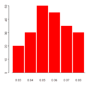
Suppose the analyst takes 200 samples, of size 300 each, from the same group of items, and achieves the following results:
Number of Samples	Percentage of Defective Items
20			3
30			4
50			5
45			6
35			7
30			8
The histogram corresponding to these results is shown below:

These results approximate a sampling distribution for the
statistic ![]() , or the distribution
of values taken by the statistic in all possible samples of the size 300
from the population of factory items. The distribution appears to be
approximately normal, with mean between 0.05 and 0.06. With repeated
sampling, the sampling distribution would more closely approximate a
normal distribution, although it would remain discontinuous because of the
granularity caused by rounding to percentage points.
, or the distribution
of values taken by the statistic in all possible samples of the size 300
from the population of factory items. The distribution appears to be
approximately normal, with mean between 0.05 and 0.06. With repeated
sampling, the sampling distribution would more closely approximate a
normal distribution, although it would remain discontinuous because of the
granularity caused by rounding to percentage points.
The variability of a statistic is determined by the spread of its sampling distribution. In general, larger samples will have smaller variability. This is because as the sample size increases, the chance of observing extreme values decreases and the observed values for the statistic will group more closely around the mean of the sampling distribution. Furthermore, if the population size is significantly larger than the sample size, then the size of the population will not affect the variability of the sampling distribution (i.e., a sample of size 100 from a population of size 100,000 will have the same variability as a sample of size 100 from a population of size 1,000,000).