Numerical Summaries
Mean
The sample mean, or average, of a group of values is calculated by taking the
sum of all of the values and dividing by the total number of values. In other words,
for n values x1, x2,
x3, ... , xn, the mean  =
(x1 + x2 + x3 + ... + xn)/n,
or

Example
Suppose a group of 10 students have the following heights (in inches):
60, 72, 64, 67, 70, 68, 71, 68, 73, 59.
The mean height for this group is
(1/10)*(60+72+64+67+70+68+71+68+73+59) = 670/10 = 67.2.
Median
The median of a group of values is the center, or midpoint, of the ordered values. The median is
calculated by placing a group of values in ascending order and taking the center observation of
the ordered list, such that there are an equal number of values above and below the median
(for an even number of observations, one may take the average of the two center values).
Example
For the data in the previous example, the median is calculated as follows:
First order the data:
59, 60, 64, 67, 68, 68, 70, 71, 72, 73.
Since there are 10 observations, the median is the average of the 5th and 6th observations,
which in this case are identical:
5th observation = 68, 6th observation = 68, median = 68.
Quartiles
The first quartile of a group of values is the value such the 25% of the values fall at or below
this value. The third quartile of a group of values is the value such that 75% of the values
fall at or below this value. The first quartile may be approximately calculated by placing a group
of values in ascending order and determining the median of the values below the true median, and
the third quartile is approximately calculated by determining the median of the values above the
true median. For an odd number of observations, the median is excluded from the calculation of
the first and third quartiles.
The distance between the first and third quartiles is known as the Inter-Quartile Range
(IQR).
A useful graphical representation of a distribution including the quartiles is a boxplot.
Example
For the data in the previous example, the quartiles may be approximately calculated as follows:
First order the data:
59, 60, 64, 67, 68, 68, 70, 71, 72, 73.
Since there are an even number of observations (10), the first half of the data is considered in calculating the first quartile:
59, 60, 64, 67, 68.
The median of these values is 64, so this is the first quartile.
The second half of the data is considered in calculating the third quartile:
68, 70, 71, 72, 73.
The median of these values is 71, so this is the third quartile.
For this example, the Inter-Quartile Range is 71-64 = 7.
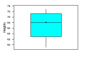
 This MINITAB boxplot corresponds to the student height data. The quartiles have been
calculated by MINITAB to represent levels for 25% and 75% of the data, with
resulting values of 63 and 71.25, respectively (see the note below for details on this calculation).
No outliers have been identified in this boxplot, since all of the observations are within
1.5*IQR from the upper and lower
quartiles.
Note: To calculate the quartiles more precisely, first multiply the percentage of interest
p by the number of observations plus one (n + 1). In our example, for 25%, this value
would be 0.25*11 = 2.75. This value lies between 2 and 3, so we wish to take a weighted average
of the 2nd and 3rd observations. The remainder of the value is 0.75, so 75% of the weight is
placed on the 3rd observation, and 100% - 75% = 25% of the weight is placed on the 2nd observation, as follows:
2nd observation = 60, 3rd observation = 64.
1st quartile = 0.25*60 + 0.75*64 = 15 + 48 = 63.
The third quartile may be calculated similarly: 0.75*11 = 8.25, so the upper quartile
lies between the 8th and 9th observation. The remainer is equal to 0.25, so 25% of the weight
is placed on the 9th observation and 75% of the weight is placed on the 8th observation.
8th observation = 71, 9th observation = 72.
3rd quartile = 0.75*71 + 0.25*72 = 53.25 + 18 = 71.25.
Variance and Standard Deviation
The variance of a group of values measures the spread of the distribution.
A large variance indicates a wide range of values, while a small variance
indicates that the values lie close to their mean. The variance s² is calculated by
summing the squared distances from each value to the mean of the values, then dividing
by one fewer than the number of observations. The standard deviation s is the
square root of the variance.

Example
The following calculation computes the variance for the student height data, where the mean was previously calculated to be 67.2:
- s² = 1/9[(59-67.2)² + (60-67.2)² +
64-67.2)² + (67-67.2)² + .... + (73-67.2)²]
- = 1/9[67.24 + 51.84 + 9.4 + 0.04 + .... + 33.64]
- = 1/9[208.76]
- = 23.2
- The standard deviation is the square root: s = 4.8.
The MINITAB "DESCRIBE" command provides a numerical summary for data which includes the mean,
median, standard deviation (abbreviated StDev), minimum and maximum values (Min and Max),
and the first and third quartiles (abbreviated Q1 and Q3). The output for our student height example
is shown below:
Descriptive Statistics

Variable        N     Mean   Median  Tr Mean    StDev  SE Mean
C1             10    67.20    68.00    67.50     4.83     1.53

Variable      Min      Max       Q1       Q3
C1          59.00    73.00    63.00    71.25
RETURN TO MAIN PAGE.
 This MINITAB boxplot corresponds to the student height data. The quartiles have been
calculated by MINITAB to represent levels for 25% and 75% of the data, with
resulting values of 63 and 71.25, respectively (see the note below for details on this calculation).
No outliers have been identified in this boxplot, since all of the observations are within
1.5*IQR from the upper and lower
quartiles.
 =
(x1 + x2 + x3 + ... + xn)/n,
or

