The Binomial Distribution
In many cases, it is appropriate to summarize a group of independent observations by the
number of observations in the group that represent one of two outcomes. For example, the
proportion of individuals in a random sample who support one of two political candidates fits
this description. In this case, the statistic
 is the count X of voters who support
the candidate divided by the total number of individuals in the group n. This provides an
estimate of the parameter p, the proportion of
individuals who support the candidate in the entire population.
The binomial distribution describes the behavior of a count variable X if
the following conditions apply:
- 1: The number of observations n is fixed.
- 2: Each observation is independent.
- 3: Each observation represents one of two outcomes ("success" or "failure").
- 4: The probability of "success" p is the same for each outcome.
If these conditions are met, then X has a binomial distribution with parameters
n and p, abbreviated B(n,p).
Example
Suppose individuals with a certain gene have a 0.70 probability of eventually contracting
a certain disease. If 100 individuals with the gene participate in a lifetime study, then the
distribution of the random variable describing the number of individuals who will contract the
disease is distributed B(100,0.7).
Note: The sampling distribution of a count variable is only well-described by the binomial
distribution is cases where the population size is significantly larger than the sample size.
As a general rule, the binomial distribution should not be applied to observations from
a simple random sample (SRS) unless the
population size is at least 10 times larger than the sample size.
To find probabilities from a binomial distribution, one may either calculate them directly,
use a binomial table, or use a computer. The number of sixes rolled by a single die in 20
rolls has a B(20,1/6) distribution. The probability of rolling more than 2 sixes
in 20 rolls, P(X>2), is equal to 1 - P(X<2) = 1 - (P(X=0) + P(X=1) +
P(X=2)). Using the MINITAB command "cdf" with subcommand "binomial n=20 p=0.166667" gives the cumulative
distribution function as follows:
Binomial with n = 20 and p = 0.166667

         x     P( X <= x)
         0        0.0261
         1        0.1304
         2        0.3287
         3        0.5665
         4        0.7687
         5        0.8982
         6        0.9629
         7        0.9887
         8        0.9972
         9        0.9994
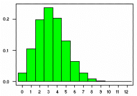
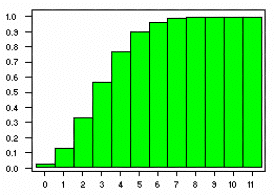
The corresponding graphs for the probability density function and cumulative distribution function
for the B(20,1/6) distribution are shown below:


Since the probability of 2 or fewer sixes is equal to 0.3287, the probability of rolling more than
2 sixes = 1 - 0.3287 = 0.6713.
The probability that a random variable X with binomial distribution B(n,p) is
equal to the value k, where k = 0, 1,....,n , is given by
 , where
  .
.
The latter expression is known as the binomial coefficient, stated as
"n choose k," or the number of possible ways to choose k "successes"
from n observations. For example, the number of ways to achieve
2 heads in a set of four tosses is "4 choose 2", or 4!/2!2! = (4*3)/(2*1) =
6. The possibilities are {HHTT, HTHT, HTTH, TTHH, THHT, THTH}, where "H" represents
a head and "T" represents a tail. The binomial coefficient multiplies the probability
of one of these possibilities (which is (1/2)²(1/2)² = 1/16 for a fair coin)
by the number of ways the outcome may be achieved, for a total probability of 6/16.
Mean and Variance of the Binomial Distribution
The binomial distribution for a random variable X with parameters
n and p represents the sum of
n independent variables Z which may assume the values 0 or 1.
If the probability that each Z variable assumes the value 1 is equal
to p, then the mean
of each variable is equal to 1*p + 0*(1-p) = p, and the
variance is equal to p(1-p). By the
addition properties for independent random variables, the mean and variance
of the binomial distribution are equal to the sum of the means and variances
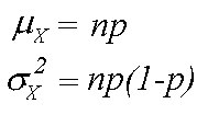
of the n independent Z variables, so

These definitions are intuitively logical. Imagine, for example, 8 flips
of a coin. If the coin is fair, then p = 0.5. One would expect the
mean number of heads to be half the flips, or np = 8*0.5 = 4. The
variance is equal to np(1-p) = 8*0.5*0.5 = 2.
Sample Proportions
If we know that the count X of "successes" in a group of n observations with
sucess probability p has a binomial distribution with mean np and variance
np(1-p), then we are able to derive information about the distribution of the
sample proportion , the count of
successes X divided by the number of observations n. By the multiplicative
properties of the mean, the mean of the distribution of X/n is equal to the mean of X
divided by n, or np/n = p. This proves that the sample proportion
 is an unbiased estimator of the population
proportion p. The variance of X/n is equal to the variance
of X divided by n², or (np(1-p))/n² = (p(1-p))/n . This formula
indicates that as the size of the sample increases, the variance decreases.
In the example of rolling a six-sided die 20 times, the probability p of rolling
a six on any roll is 1/6, and the count X of sixes has a B(20, 1/6) distribution.
The mean of this distribution is 20/6 = 3.33, and the variance is 20*1/6*5/6 = 100/36 = 2.78.
The mean of the proportion of sixes in the 20 rolls, X/20, is equal to
p = 1/6 = 0.167, and the variance of the proportion is equal to (1/6*5/6)/20 = 0.007.
Normal Approximations for Counts and Proportions
For large values of n, the distributions of the count X and the sample proportion
 are approximately normal.
This result follows from the Central Limit Theorem.
The mean and variance for the approximately normal distribution of X are np
and np(1-p), identical to the mean and variance of the binomial(n,p) distribution.
Similarly, the mean and variance for the approximately normal distribution of the sample
proportion are p and (p(1-p)/n).
Note: Because the normal approximation is not accurate for small values of n, a good rule of
thumb is to use the normal approximation only if np>10 and
np(1-p)>10.
For example, consider a population of voters in a given state. The true proportion of voters who
favor candidate A is equal to 0.40. Given a sample of 200 voters, what is the probability that
more than half of the voters support candidate A?
The count X of voters in the sample of 200 who support candidate A is distributed
B(200,0.4). The mean of the distribution is equal to 200*0.4 = 80, and the variance is equal
to 200*0.4*0.6 = 48. The standard deviation is the square root of the variance, 6.93. The
probability that more than half of the voters in the sample support candidate A is equal to
the probability that X is greater than 100, which is equal to 1- P(X< 100).
To use the normal approximation to calculate this probability, we should first acknowledge that
the normal distribution is continuous and apply the continuity correction.
This means that the probability for a single discrete value, such as 100, is extended to the
probability of the interval (99.5,100.5). Because we are interested in the probability
that X is less than or equal to 100, the normal approximation applies to the upper limit
of the interval, 100.5. If we were interested in the probability that X is strictly less
than 100, then we would apply the normal approximation to the lower end of the interval, 99.5.
So, applying the continuity correction and standardizing the variable X gives the following:
1 - P(X< 100)
= 1 - P(X< 100.5)
= 1 - P(Z< (100.5 - 80)/6.93)
= 1 - P(Z< 20.5/6.93)
= 1 - P(Z< 2.96) = 1 - (0.9985) = 0.0015. Since the value 100 is nearly three
standard deviations away from the mean 80, the probability of observing a count this high is
extremely small.
RETURN TO MAIN PAGE.
 , where
  .
.
