Inference in Linear Regression
Linear regression attempts to model the relationship between two variables by fitting a linear
equation to observed data. Every value of the independent variable x is associated with
a value of the dependent variable y. The variable y is assumed to be normally distributed with mean  y and
variance
  . The least-squares regression line
y = b0 + b1x is an estimate of the true population
regression line,
  y
=
y
=  0 +
0 +  1x.
This line describes how the mean response
 y changes with x. The observed values for
y vary about their means
  y and are assumed
to have the same standard deviation
  . The
fitted values b0 and b1 estimate the true intercept and
slope of the population regression line.
Since the observed values for y vary about their means  y,
the statistical model includes a term for this variation. In words, the model is expressed
as DATA = FIT + RESIDUAL, where the "FIT" term represents the expression
  0 +
0 +
 1x.
The "RESIDUAL" term represents the deviations of the observed values y from their
means
  y, which are normally distributed with mean
0 and variance
  . The notation for the model deviations is
 .
.
In formal terms, the model for linear regression is the following:
Given n pairs of observations (x1, y1),
(x2, y2), ... , (xn, yn), the
observed response is yi =  0 +
0 +
 1xi
+
1xi
+  i.
i.
In the least-squares model, the best-fitting line for the observed data is calculated by
minimizing the sum of the squares of the
vertical deviations from each data point to the line (if a point lies on the fitted line exactly,
then its vertical deviation is 0). Because the deviations are first squared, then summed, there
are no cancellations between positive and negative values. The least-squares estimates
b0 and b1 are usually computed by statistical software. They
are expressed by the following equations:
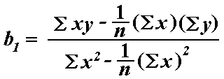

The computed values for b0 and b1 are unbiased estimators
of  0 and
0 and  1, and are normally distributed with standard deviations
that may be estimated from the data.
The values fit by the equation b0 +
b1xi are denoted  i, and the residuals ei are equal to
yi -
  i, the difference between the observed and fitted values.
The sum of the residuals is equal to zero.
The variance  ² may be estimated by s² =
 , also known as the mean-squared error (or MSE).
The estimate of
the standard error s is the square root of the MSE.
Example
The dataset "Healthy Breakfast" contains, among other variables,
the Consumer Reports ratings of 77 cereals and the number of grams of sugar contained
in each serving. (Data source: Free publication available in many grocery stores.
Dataset available through the Statlib Data and Story Library (DASL).)
The correlation between the two variables is -0.760, indicating a strong
negative association. A scatterplot of the two variables indicates
a linear relationship:
Using the MINITAB "REGRESS" command with "sugar" as an explanatory variable and "rating"
as the dependent variable gives the following result:
Regression Analysis

The regression equation is
Rating = 59.3 - 2.40 Sugars
A plot of the data with the
regression line added is shown to the right: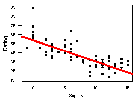
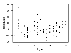
After fitting the regression line, it is important to investigate the residuals to determine
whether or not they appear to fit the assumption of a normal distribution. A plot of the
residuals y -  on the vertical axis with the corresponding explanatory values
on the horizontal axis is shown to the left. The residuals do not seem to deviate from a random
sample from a normal distribution in any systematic manner, so we may retain the assumption of
normality.
The MINITAB output provides a great deal of information. Under the equation for the
regression line, the output provides the least-squares estimate for the constant b0
and the slope b1. Since b1 is the coefficient of the explanatory
variable "Sugars," it is listed under that name. The calculated standard deviations for the
intercept and slope are provided in the second column.
Predictor       Coef       StDev          T        P
Constant      59.284       1.948      30.43    0.000
Sugars       -2.4008      0.2373     -10.12    0.000

S = 9.196       R-Sq = 57.7%     R-Sq(adj) = 57.1%
Significance Tests for Regression Slope
The third column "T" of the MINITAB "REGRESS" output provides test statistics.
In linear regression, one wishes to test the
significance of the parameter included. The null hypothesis states that
the slope coefficient,  1, is equal to 0.
If this is true, then there is no linear relationship between the explanatory and dependent
variables -- the equation y =
  0 +
0 +
 1x
+
1x
+  simply becomes y =
 0 +
0 +
 .
The alternative hypothesis may be one-sided or two-sided, stating
that
  1
is either less than 0, greater than 0, or simply not equal to 0.
The test statistic t is equal to b1/sb1,
the slope parameter estimate
divided by its standard deviation. This value follows a t(n-2) distribution.
In the example above, the slope parameter estimate is -2.4008 with standard deviation
0.2373. The test statistic is t = -2.4008/0.2373 = -10.12, provided in the "T" column of
the MINITAB output. For a two-sided test, the probability
of interest is 2P(T>|-10.12|) for the t(77-2) = t(75) distribution,
which is an extremely small value. The "P" column of the MINITAB output provides the P-value
associated with the two-sided test.
Condidence Intervals for Regression Slope and Intercept
A level C confidence interval for the parameters  0
and
0
and  1
may be computed from the estimates b0 and b1 using the
computed standard deviations and the appropriate critical value t* from
the t(n-2) distribution. The confidence interval for
  0
takes the form b0 + t*sb0, and the confidence interval
for
  1 is given by b1 + t*sb1.
In the example above, a 95% confidence interval for the slope parameter  1
is computed to be (-2.4008 + 2.000*0.2373) = (-2.4008 - 0.4746, -2.4008 + 0.4746)
= (-2.8754, -1.9262).
The value for "S" printed in the MINITAB output provides the estimate for the standard deviation
 , and the "R-Sq" value is the square of the correlation r
written as a percentage value. This indicates the 57.7% of the variability in the cereal ratings
may be explained by the "sugars" variable.
Confidence Intervals for Mean Response
The mean of a response y for any specific value of x,
say x*, is given by  y
=
y
=  0 +
0 +
 1x*. Substituting the fitted
estimates b0 and b1 gives the equation
 y = b0 +
b1x*. A confidence interval for the mean response is calculated
to be
  y + t*s
 , where the fitted value
 y is
the estimate of the mean response. The value t* is the upper (1 - C)/2
critical value for the t(n - 2) distribution.
The MINITAB "BRIEF 3" command expands the output provided by the "REGRESS" command to include
the observed values of x and y, the fitted values
 y, the standard deviation of the fitted values (StDev Fit), the residual values,
and the standardized residual values. The table below shows this output for the first 10
observations.
Obs    Sugars     Rating        Fit  StDev Fit   Residual    St Resid
  1       6.0      68.40      44.88       1.07      23.52       2.58R
  2       8.0      33.98      40.08       1.08      -6.09      -0.67
  3       5.0      59.43      47.28       1.14      12.15       1.33
  4       0.0      93.70      59.28       1.95      34.42       3.83R
  5       8.0      34.38      40.08       1.08      -5.69      -0.62
  6      10.0      29.51      35.28       1.28      -5.77      -0.63
  7      14.0      33.17      25.67       1.98       7.50       0.84
  8       8.0      37.04      40.08       1.08      -3.04      -0.33
  9       6.0      49.12      44.88       1.07       4.24       0.46
 10       5.0      53.31      47.28       1.14       6.03       0.66
To compute a confidence interval for the mean response of an observation, first choose a critical
value from the appropriate t distribution. For a 95% confidence interval, the t(75)
critical value is approximately 2.000. For the second observation in the table above,
a 95% confidence interval for the mean response is computed to be (40.08 + 2.000*1.08)
= (40.08 + 2.16) = (37.92, 42.24).
Prediction Intervals
Once a regression line has been fit to a set of data, it is common to use the fitted slope
and intercept values to predict the response for a specific value of x,
say x*, that was not included in the original set of observations. The estimate
for the response  is identical to the estimate for
the mean of the response:
  = b0 +
b1x*. The confidence interval for the predicted value is given by
 + t*s
+ t*s , where
 is the fitted value corresponding to x*.
The value t* is the upper (1 - C)/2
critical value for the t(n - 2) distribution.
Note:The standard error associated with
a prediction interval is larger than the standard deviation for the mean response, since
the standard error for a predicted value must account for added variability.
The MINITAB "PREDICT" subcommand computes the predicted response variable and provides 95%
confidence limits. Suppose we are interested in predicting the rating for a cereal with a
sugar level of 5.5. MINITAB produces the following output:
     Fit  StDev Fit       95.0% CI             95.0% PI
   46.08       1.10   (   43.89,   48.27)  (   27.63,   64.53)
The fitted value 46.08 is simply the value computed when 5.5 is substituted into the equation
for the regression line: 59.28 - (5.5*2.40) = 59.28 - 13.20 = 46.08. The value given in the
95.0% CI column is the confidence interval for the mean response, while the value given
in the 95.0% PI column is the prediction interval for a future observation.
For additional tests and a continuation of this example, see ANOVA
for Regression.
RETURN TO MAIN PAGE.
 y,
the statistical model includes a term for this variation. In words, the model is expressed
as DATA = FIT + RESIDUAL, where the "FIT" term represents the expression
  0 +
0 +
 1x.
The "RESIDUAL" term represents the deviations of the observed values y from their
means
  y, which are normally distributed with mean
0 and variance
  . The notation for the model deviations is
 .
.


 , also known as the mean-squared error (or MSE).


 y = b0 +
b1x*. A confidence interval for the mean response is calculated
to be